
Statistical Decisions Hellas S.A. (StatDec), a niche consulting specializing in credit risk analytics and data-driven decision models, with over 30 years of experience supporting financial institutions in Greece and abroad, announces its acquisition by Tiresias S.A., the only Credit Bureau in Greece and a member of the Association of Consumer Credit Information Suppliers (ACCIS).
Through this strategic partnership, StatDec becomes the consulting arm of Tiresias, enhancing the overall value proposition offered to market participants. Under the agreement, StatDec will continue to operate as a distinct entity and as a member of the Tiresias S.A. Group.
The affiliation of the two companies creates significant synergies, enabling the provision of comprehensive risk management and consulting services to the financial sector, businesses, and individuals. StatDec will continue to serve its clients with the same professionalism and commitment, while leveraging the scale and resources of Tiresias to deliver innovative, high–value-added tools and services.
Mr. Nikolas Karanasios Chief Executive Officer of StatDec, stated:
“Tiresias’ investment in StatDec marks a strategic step forward, creating a new value proposition in the market. By combining StatDec’s expertise in consulting and analytics with Tiresias’ unique data and know-how in credit risk assesment, we are equipped to deliver even more reliable and impactful solutions to our clients.”
Mr. Ilias Xirouhakis, Chief Executive Officer of Tiresias SA, stated:
“By acquiring StatDec, Tiresias takes a bold step towards becoming a world class Credit Bureau, providing modern data analytics services and risk management consulting services. The acquisition is a considerable investment in the responsible financing of businesses and individuals and as such, in the sustainability of the Greek economy, further strengthening the institutional role of Tiresias."

The covid-19 pandemic has turned many economies into recession, the duration and depth of which is unknown and still debated. Initially a V shape recovery was the popular narration among economists. By mid April, when this analysis is written, a U shape impact gains the consensus, with the adverse L type scenario being described as less likely.
Most countries have taken multiple tiered measures to relief their citizens from the sudden and sharp fall of economic activity. Among them was the implementation of a moratorium of payments on loans held by individuals and businesses.
European Banking Authority, at their merit, demonstrated quick reflexes, by issuing statement and then guidance on default recognition eligibility and specifications over Significant Increase in Credit Risk (SICR) in case of payments moratorium.
The payments moratorium, however, will affect all the components of the Expected Credit Loss function in a variety of ways.
PD and Lifetime PD estimates
Most PD and Lifetime PD (LPD) retail estimates are based on Behaviour Scores or behaviour related attributes. In case of a business as usual classification of exposures continues during moratorium, the following dynamics are expected:
- Delinquency Bucket based predictors will demonstrate an artificially improved picture, i.e. with no delays in the behaviour period
- Payment counters / balance change related predictors on the other side will suggest an increase in risk levels
Given that bucket-based criteria are usually the predominant drivers in risk classifications, the overall expectation would be a concentration of the exposures (due to their characteristics becoming static) and a shift towards best PD pools (due to the higher importance of bucket related predictors). The higher the participation rate in the moratorium, the more intense these dynamics are expected to be as is presented in the following visualisation. In fact, these effects are expected to continue in the first months following the end of moratorium, until payment behaviour history is restored.
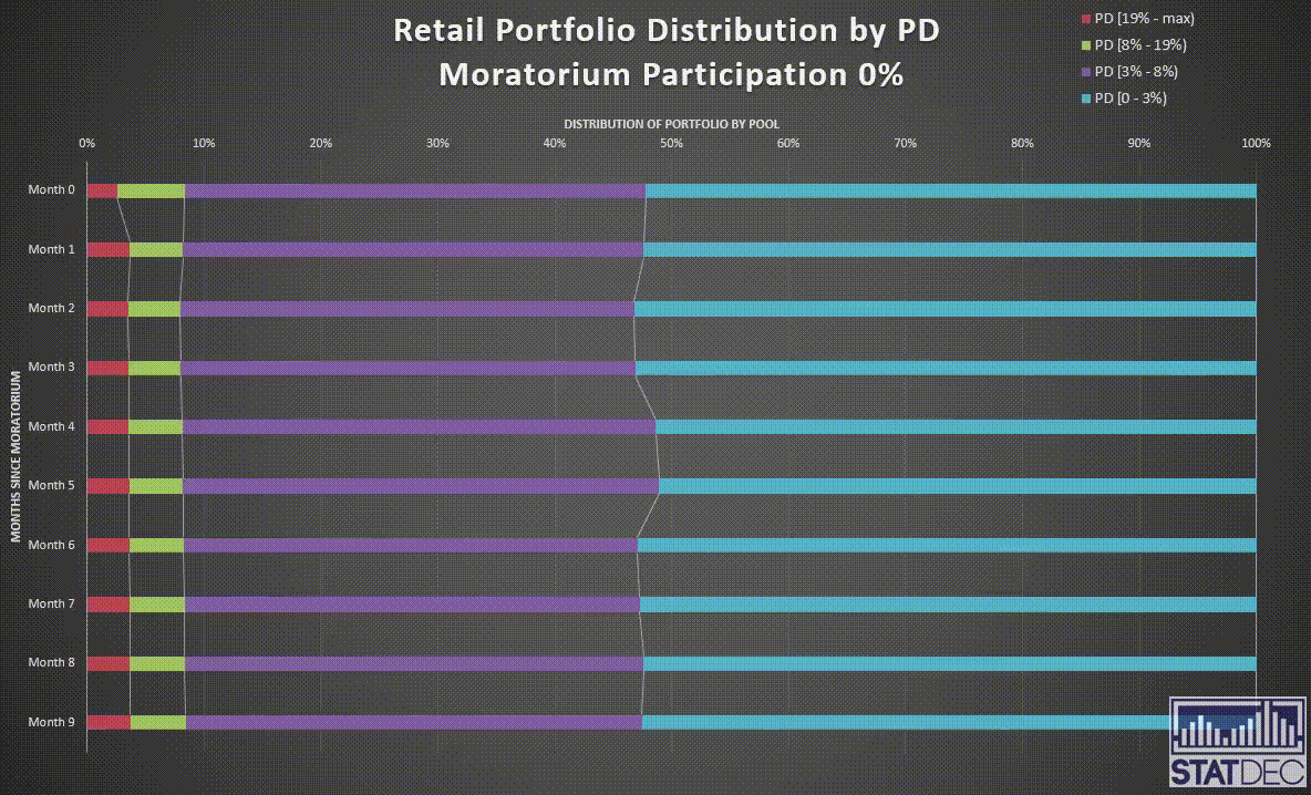
Beyond doubt, those patterns are not representing the true status of the portfolio. The overall risk level of the portfolio is not reducing, the classification is misleading and relationship between PD Pools and PD is not yet known.
Though each situation may be different, the general objective is to perform a classification considering the credit risk profile of the client and the level of exposure to the risks of the current economic environment in mid-term period, i.e. when the moratorium is expected to end. This could be achieved by combining
- A frozen version of the PD pools (or Behaviour Scores) before the impact of covid-19, which would represent credit risk profile
- With the forecasted impact of covid-19 by sector/type of activity
This approach introduces a forward looking aspect in the PD estimates and may have various levels of complexity, i.e. in the way the combination takes place (score level, overlay etc.), in the level of judgmental decision and use of any relevant historical data, fresh data as become available or by generalizing relations identified in economic sectors in other countries.
LGD estimates
The Cure Rate component of the Loss Given Default (LGD) estimates is where the main interest needs to be placed, as is more sensitive to economic conditions while most remedial strategies are focusing in increasing cure rates.
Cure Rates are expected to be impacted in the following matters:
- Exposures being in default for less than 12 months (new defaults), for which usually a higher cure rate is expected, will be affected the most. For these exposures, the ability to make payments and become current is greatly impaired by the distressed economic conditions. Thus, the 12-month cure rate should be readjusted downwards. If a macro layer exists for this component, it could be employed considering the macroeconomic projections for GDP and other macroeconomic variables. If not, stressing the estimate is recommended. However, depending on the shape of the economic recovery, cure rates of the subsequent period may be significantly higher than any past observation. As such pattern may not be available in any training data for producing the estimate, Cure Rate in 2021 for months in default 13-24 may exceed any pre-existing macro-based model estimate.
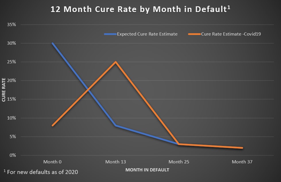
- For exposures currently 13 months or more in default, expected cure rates should as well be downward adjusted, while expectations of cure rate bouncing in 2021 (i.e. at 25+ month in default by then) are low.
- Exposures not in default (stage 1 and 2) may be classified in two categories:
- For exposures eligible or in the moratorium, any default event will occur after the moratorium (with the exception of unlikeliness to pay (UTP) triggered default). The macroeconomic projections for this period (2021) are in most cases favorable. To a degree, Cure estimates as the existing or similar may be close to reality.
- For exposures not eligible for moratorium, the expected pattern should be similar to the already defaulted exposures (orange line in the previous chart), in case of default.
- Regarding expected recoveries from properties realization, property indexes should be adjusted according to scenarios on recession type that will impact the economy.
- Cash recoveries usually refer to a longer-term recovery period so less impact is expected
- It also worth noticing the need for extension of probation for already forborne exposures eligible for moratorium.
EAD estimates
Exposure at Default (EAD) estimates are expected to be impacted only mildly by the covid-19 and moratorium measures. Main dynamics that can be expected are:
- For fixed term exposures, the prolongation of the term with capitalization of interest should be considered in the estimated EAD in the term structure.
- For revolving, as long as limit monitoring, cash advances and authorizations tracking are in place, no impact is expected. It worth noticing though that in recession periods, inactive revolving facilities may become activated, with high default rates and high limit usages.
Conclusion
The first step for responding to the new reality that covid-19 introduced and the economic recession expected for 2020 is to understand and predict how the portfolios will be affected. Only then can decisions be informed, and appropriate actions can be taken so as to manage portfolios through these difficult circumstances.Towards this direction, adjustments or calibration of the ECL components estimates will be required, probably along with a further level of granularity that will better depict expectations for a different size effect on particular segments.
Portfolio analysis is undertaken to determine whether the present and expected future losses are consistent with the revenue expectations of the portfolio and enable it to generate a profit both now and in the future.
The phrase loss minimisation is not used since losses and revenue are closely linked in many products; nowhere more so that in credit cards and lines of credit.
The transition from a current, interest earning, account to a credit loss takes place via a series of different levels of delinquency. It is the analysis between these different levels of delinquency over time which form the core of the analysis.
Start with Objective Measures
The whole process falls apart if the measure of delinquency is not objective and consistent. Yet it is surprising how often this is the case amongst many of our leading consumer banks.
Issues include, amongst others:
- Erratic treatment of partial or multiple payments
- Loan rescheduling accompanied by re-setting of delinquency status and without separate monitoring
- Inconsistent treatment of fee payments
- Collector intervention in the ageing process.
Analysis that is performed on inaccurate data is like a house built without foundations. It is likely to fall down.
Monthly Delinquency Reports
It is common to report the status of a portfolio broken down into the different levels of delinquency as measured by contractual ageing. (That is the number of days delinquent is measured against the schedule established when the credit agreement was signed and the amount reported is the balance, shown as the “balance at risk” (net of any unearned income)).
| Delinquency | Jan - 21 |
| Current | 1,234,567 |
| 1 29 dpd | 49,383 |
| 30 59 dpd | 11,358 |
| 60 89 dpd | 4,998 |
| 90 119 dpd | 3,798 |
| 120 149 dpd | 3,342 |
| 150 179 dpd | 2,975 |
| 180 209 dpd | 2,796 |
| 210 239 dpd | 2,712 |
| 240-269 dpd | 2,658 |
| 270 299 dpd | 2,631 |
| 300 329 dpd | 2,605 |
| 330 359 dpd | 2,579 |
| .. | .. |
| 720 dpd | 2,566 |
A report of this kind will look like the one above. The numbers used are realistic for a mature portfolio. In the example we have drawn a line across the table at 180 days past due which is the point at which the accounts are written–off.
Write-off is often mistakenly understood to mean that there will be no future revenue from the account. In fact in most markets there is still significant value of an account that has been written-off. The debt for the customer still stands and there is still a legal obligation on behalf of the customer to settle the debt. The extent to which they are collected depends very much on either the local legal environment or the efforts of the collector. In countries, such as Germany, where it is usual for banks to apply to the courts for a portion of the customers wages to be assigned directly to the bank the rate of recovery can be very high. Where this legal support is not available the proportion collected will depend on the skill of the collections department and usually varies between 0% and 33%.
In most countries there is an active market for the sale of written-off debt with prices varying up to a maximum of around 8% of the face value of the debt. The logic for this maximum is that if the debt is recoverable at 33% then the cost of recovery will typically be less than 25%.
In our example the delinquency may not be important in terms of the reported results of a business but for the credit risk manager understanding the evolution of delinquency beyond write-off is critical.
Of the balances which are not written-off it is normal to consider the ratios of the percentage of balances which are greater than 30dpd and the percentage greater than 90dpd. In the case of our example the ratios are
30+ dpd delinquency - 2.2%
90+ dpd delinquency - 1.0%
The percentage of the receivable written-off in a given month which is called the gross credit write-off is 0.21%. If this is repeated in every month of the year the annual gross write-off would be 12 x 0.21% or 2.52%.
Static to Dynamic Delinquency
Although these numbers are commonly used they shed very little light on any possible cause of delinquency nor upon the impact of any changes in the portfolio.
If the delinquency figures for two consecutive months are written side by side then a direct comparison can be made between the two months. In the table underneath can be seen that not only are the receivables growing but so are the delinquent balances at each level of delinquency.
Unfortunately the table doesn’t say anything about the movement of accounts between the two months so accounts which for example, are 1-29dpd in Feb-21 may have been in any non-written-off bucket in January.
Of course the maximum an account can age between two months is 30 days but they can pay off as much of the overdue balance as they are able and can become less delinquent all the way back to current or anywhere in between.
Experience, however, tells us that the evolution of delinquency for accounts beyond 60 dpd is likely to be determined primarily by most customers making no payment and simply ageing to the next bucket.
| Delinquency | Jan-21 | Feb-21 |
| Current | 1,234,567 | 1,296,295 |
| 1 - 29 dpd | 49,383 | 61,728 |
| 30 59 dpd | 11,358 | 12,346 |
| 60 89 dpd | 4,998 | 5,111 |
| 90 119 dpd | 3,798 | 3,748 |
| 120 149 dpd | 3,342 | 3,228 |
| 150 179 dpd | 2,975 | 3,008 |
| 180 209 dpd | 2,796 | 2,826 |
| 210 239 dpd | 2,712 | 2,740 |
| 240 269 dpd | 2,658 | 2,658 |
| 270 299 dpd | 2,631 | 2,605 |
| 300 329 dpd | 2,605 | 2,579 |
| 330 359 dpd | 2,579 | 2,553 |
| .. | .. | .. |
| .. | .. | .. |
| 720 dpd | 2,566 | 2,566 |
It suits our purpose to make the simplifying assumption that all accounts arriving in a given delinquency bucket come from the previous (one lower) stage of delinquency. This assumed movement from month to month is called the “net flow” or “roll” of delinquent balances.
From the above table we will be saying that the flow from the 30-59dpd bucket in January to the 60-89dpd bucket in February is 11,358 -> 5,111 or a flow of 45%.With this simplifying assumption in place it becomes possible to analyse further what is happening to risk within a portfolio.
The Net Flow Matrix
On the following two tables, the first is a delinquency matrix which shows the balances delinquent for a series of 12 months, whilst the second table is a net flow matrix which shows the transition to a state of delinquency in a given month from a state of lower delinquency in the previous month under the assumption that accounts either only become one step more delinquent every month or cure entirely (a simplification but adequate especially for the later buckets).
| Delinquency | Jan-21 | Feb-21 | Mar-21 | Apr-21 | May-21 | Jun-21 | Jul-21 | Aug-21 | Sep-21 | Oct-21 | Nov-21 | Dec-21 |
| Current | 1,234,567 | 1,296, 295 | 1,361,110 | 1,429,166 | 1,500,624 | 1,575,655 | 1,654,438 | 1,737,160 | 1,824,018 | 1,915,219 | 2,010,980 | 2,111,529 |
| 1 - 29 dpd | 49,383 | 61,728 | 64,815 | 68,056 | 71,458 | 75,031 | 78,783 | 82,722 | 86,858 | 91,201 | 95,761 | 100,549 |
| 30 - 59 dpd | 11,358 | 12,346 | 15,432 | 16,204 | 17,014 | 17,865 | 18,758 | 19,696 | 20,680 | 21,714 | 22,800 | 23,940 |
| 60 - 89 dpd | 4,998 | 5,111 | 5,556 | 6,944 | 7,292 | 7,656 | 8,039 | 8,441 | 8,863 | 9,306 | 9,772 | 10,260 |
| 90 - 119 dpd | 3,798 | 3,748 | 3,833 | 4,167 | 5,208 | 5,469 | 5,742 | 6,029 | 6,331 | 6,647 | 6,980 | 7,329 |
| 120 - 149 dpd | 3,342 | 3,228 | 3,186 | 3,258 | 3,542 | 4,427 | 4,648 | 4,881 | 5,125 | 5,381 | 5,650 | 5,933 |
| 150 - 179 dpd | 2,975 | 3,008 | 2,906 | 2,867 | 2,932 | 3,187 | 3,984 | 4,184 | 4,393 | 4,612 | 4,843 | 5,085 |
| 180-209 dpd | 2,796 | 2,826 | 2,858 | 2,760 | 2,724 | 2,786 | 3,028 | 3,785 | 3,974 | 4,173 | 4,382 | 4,601 |
| 210 - 239 dpd | 2,712 | 2,740 | 2,769 | 2,801 | 2,705 | 2,669 | 2,730 | 2,968 | 3,709 | 3,895 | 4,090 | 4,294 |
| 240-269 dpd | 2,658 | 2,658 | 2,685 | 2,714 | 2,745 | 2,651 | 2,616 | 2,676 | 2,908 | 3,635 | 3,817 | 4,008 |
| 270 - 299 dpd | 2,631 | 2,605 | 2,605 | 2,632 | 2,660 | 2,690 | 2,598 | 2,564 | 2,622 | 2,850 | 3,563 | 3,741 |
| 300 - 329 dpd | 2,605 | 2,579 | 2,553 | 2,553 | 2,579 | 2,607 | 2,636 | 2,546 | 2,512 | 2,570 | 2,793 | 3,491 |
| 330 - 359 dpd | 2,579 | 2,553 | 2,527 | 2,502 | 2,502 | 2,528 | 2,554 | 2,583 | 2,495 | 2,462 | 2,518 | 2,737 |
| .. | .. | .. | .. | .. | .. | .. | .. | .. | .. | .. | .. | .. |
| 720 + dpd | 2,566 | 2,566 | 2,566 | 2,566 | 2,566 | 2,566 | 2,566 | 2,566 | 2,566 | 2,566 | 2,566 | 2,566 |
| Jan-21 | Feb-21 | Mar-21 | Apr-21 | May-21 | Jun-21 | Jul-21 | Aug-21 | Sep-21 | Oct-21 | Nov-21 | Dec-21 | |
| 1 - 29 dpd | 5% | 5% | 5% | 5% | 5% | 5% | 5% | 5% | 5% | 5% | 5% | |
| 30 - 59 dpd | 25% | 25% | 25% | 25% | 25% | 25% | 25% | 25% | 25% | 25% | 25% | |
| 60 - 89 dpd | 45% | 45% | 45% | 45% | 45% | 45% | 45% | 45% | 45% | 45% | 45% | |
| 90 - 119 dpd | 75% | 75% | 75% | 75% | 75% | 75% | 75% | 75% | 75% | 75% | 75% | |
| 120 - 149 dpd | 85% | 85% | 85% | 85% | 85% | 85% | 85% | 85% | 85% | 85% | 85% | |
| 150 - 179 dpd | 90% | 90% | 90% | 90% | 90% | 90% | 90% | 90% | 90% | 90% | 90% | |
| 180 - 209 dpd | 95% | 95% | 95% | 95% | 95% | 95% | 95% | 95% | 95% | 95% | 95% | |
| 210 - 239 dpd | 98% | 98% | 98% | 98% | 98% | 98% | 98% | 98% | 98% | 98% | 98% | |
| 240-269 dpd | 98% | 98% | 98% | 98% | 98% | 98% | 98% | 98% | 98% | 98% | 98% | |
| 270 - 299 dpd | 98% | 98% | 98% | 98% | 98% | 98% | 98% | 98% | 98% | 98% | 98% | |
| 300 - 329 dpd | 98% | 98% | 98% | 98% | 98% | 98% | 98% | 98% | 98% | 98% | 98% | |
| 330 - 359 dpd | 98% | 98% | 98% | 98% | 98% | 98% | 98% | 98% | 98% | 98% | 98% | |
| .. | .. | .. | .. | .. | .. | .. | .. | .. | .. | .. | .. | .. |
| 720 + dpd | 2,566 | 2,566 | 2,566 | 2,566 | 2,566 | 2,566 | 2,566 | 2,566 | 2,566 | 2,566 | 2,566 | 2,566 |
The net flow tells quite a detailed story about how the portfolio is being managed. First of all the evolution of an account through the different stages of delinquency gives the monthly gross loss (before recoveries). The simplest way of stating this is to say that the losses which arrive at 180 dpd in August 2021 were current in January of that year. So the percentage that becomes written-off from that month is 3,785 / 1,234,567 or 0.306% of the current balance. If this happens on each of 12 months of the year then the annualised loss rate is 3.68% of the current balance.
Another way of calculating the same number is to take the product of the monthly flows:
5% x 25% x 45% x 75% x 85% x 90% x 95% = 0.306%
The advantage of this way of looking at things is that it breaks the losses down into different stages of the evolution and if there is deterioration in any part of the process it can be quickly identified and remedial actions taken.
If the losses were to deteriorate by 20% from 0.306% per month to 0.366% per month then the reason may not be obvious immediately, however if it can be seen that the flow rates have changed to those underneath
5% x 25% x 54% x 75% x 85% x 90% x 95% = 0.366%
It can be seen that the flow from the 30pd bucket to the 60dpd bucket has increased from 45% to 54%, which accounts for the 20% increase in the gross losses. The problem lies in a specific part of the collections area. It could be due to staff shortages or some other such change in collections strategy but at least the problem has been located and can be treated.
Breaking the Flow
It has become common practice for lots of good reasons to break the transition from current good customer to recognised final loss into a number of stages. This is partially encapsulated in Basel II where the division is made between account prior to default (usually 90 dpd) and post default. This enables the Basel II formulation of expected losses as:
EL=PD x LGD x EAD
Many lenders would provide a more detailed breakdown of the process divining the loss given default transition into two separate parts; that prior to write-off and that post write-off.
This is because experience tells us that the analysis for predicting write-off from delinquent status works quite well using a net flow model but beyond that it is better to perform vintage analysis to forecast future losses.
The other major advantage of this kind of analysis is that it can be used to understand the true state of the portfolio without being misled by the impact of the effects of growth.
In the example that we are looking at on the previous page the accountants view of the percentage of losses would simply be the balances written-off divided by the sum of the previously non written-off balances. This is 0.203% of total balance (0.218% of current balance) or almost a third lower than the lagged value.
This is because the receivable that is used as the denominator refers to the month of the write-off. Since the portfolio has been growing since the time when the newly written-off account was current the denominator is higher and the ratio of losses is lower. Of course if the situation is reversed then the denominator shrinks and the loss ratio becomes higher.
A growing portfolio can conceal a multitude of problems and care needs to be taken to analyse its true quality.
Concepts on the Measurement of Loss
Another difference in the calculations is not related to the lagging factor but to the denominators used. The lagged flow gives a loss rate as a percent of the lagged current balance while the accountants’ loss rate is this month’s written-off balance as a percent of this month’s not previously written-off balances. In both approaches, this is a simplification with the lagged calculation assuming receivables only from current bucket and the standard approach total receivables. In reality losses should be measured as a percentage of performing, interest earning assets.
The lagged calculation could be seen as more prudent as it looks at only the major portion of interest earning balances and removes the effects of growth. The accountant’s simplified view of the world has an account as either performing or written-off and confuses numerators and denominators.
A more accurate calculation, however, would use a risk weighting/impairment on all buckets as delinquent balances, although still considered as assets, have a much diminished potential for earning interest.
Conclusions
The challenging part of the risk analysis is not the preparation of the data, although inaccurate data makes any analysis impossible, it is in the interpretation of that data.
The whole management process is geared to producing a profitable portfolio and the credit process must be designed to be consistent with this. This means to have an understanding of what are the acceptable level of losses and knowing what are the revenues and costs associated with a given product.
Once that is established the whole lending process from underwriting through limit setting, maintenance and collections must function in order to achieve the acceptable level of risk.

From 1st January 2021 the new guidelines on the application of the definition of default (EBA/GL/2016/07) are in effect in all EU countries. The purpose of the guidelines is to ensure a common and consistent definition of default across institutions not only under the same local supervisor but also across EU countries. One key component of interest is the introduction of a new standard on the materiality rule for the past due criterion in counting of days past due and the identification of default.
Our experience from credit portfolios in many countries also confirms that there is a diversity of implemented versions of the past due criteria making EBA’s view to establish a common ground reasonable. However, the requirements bring new dynamics and additional challenges for the financial institutions. In this article, we are discussing about the patterns introduced under the new definition, the potential impact on the Bank’s portfolios and models, while we also look at the applicability of the definition in making business decisions.
The New Standard on Counting Delinquency
Among other changes, under the new definition, the counting of days past due begins from the moment when the sum of the past due amounts breaches the relative and absolute thresholds. This approach of counting days past due shows the following main characteristics:
- There is a delay in the identification of delinquencies and defaults as the counter begins when the total past due amount becomes material.
- The counter continues to increase even in the case of some repayments of past due amounts as long as both thresholds being breached.
The following table presents an example of a retail non-forborne mortgage loan.

The table provides a comparison between the past due criterion under the new definition and the past due counter before the new changes. We will use this as an example to highlight the ‘path to default’ in both definitions. In the example, both materiality thresholds under the new definition are breached on 07/2021 and the material past due counter begins counting while it needs additional time to trigger the default event. Despite the regular payments of past due amounts, the exposure continues to be delinquent as the remaining past amounts still breach the materiality thresholds. After full repayment of the overdue amount is made, it takes additional 3 months to exit NPE status due to the probation period introduced with the new default exit criteria.
On the contrary, the existing past due counter shows delinquent behavior from the first unpaid amount while never reaches non-performing status (90+ DPD), irrespective of materiality threshold used in default definition, due to the regular repayments of past due amounts.
Portfolio Impact
The introduction of the new definition of default in retail portfolios may impact to a varying degree all aspects of credit risk modelling and reporting. The effect in terms of non-technical defaults can be complicated and depends on the definition that each institution had already in use before complying with the new standard.
Distribution Impact
Figure 1 presents the distribution of exposures at each DPD group (bucket) for a retail mortgage portfolio comparing the new DPD against the existing DPD calculation.

Figure 2 provides the compound flow rate to bucket 4 from a given current delinquent state.

Figure 3 presents the flow rate to subsequent buckets.

The main points to consider are:
- The materiality thresholds in days past due counting create a higher concentration of exposures in the 0 DPD group (“Bucket 0”) relative to the existing DPD counting, when delinquent amounts fail to exceed both thresholds.
- For the new material DPD, when the past due amount remains above the thresholds, delinquency buckets 1-3 are only transitory stages in which an exposure either continues to higher delinquency buckets reaching eventually non-performing status or transits to current status if adequate repayments are made. The transitory behavior of the new material DPD is evident in graphs 2 & 3 where on average there is higher flow rate to subsequent buckets and ultimately to bucket 4 state under the new DPD counting compared to the existing one.
- The lower proportion of bucket 0 population and their higher flow to bucket 1 depict the early warning nature of the existing DPD counting as it can identify payment difficulties even before they become material.
Impact on Risk Profile
The following table shows the default rates based on the new DoD for the ‘Bucket 0’ population under the new DPD counting by segments of the existing DPD counting (existing delinquency buckets) for a retail mortgage portfolio.

The table shows a contamination effect especially under the new definition. The higher concentration of exposures in the bucket 0 conceals segments of the portfolio with riskier profile. The existing past due counter is able to identify riskier segments mainly because can indicate exposures with missed payments before the total past due amount becomes material under the new definition. Using a combination of the new materiality DPD counter with a more traditional DPD counter could potentially identify portfolio segments with different risk profiles creating more robust rating systems.
Business Impact
By design, the new definition of default reflects on supervisors’ objectives and point of view, leaning towards to a more conservative approach of classification of NPE exposures. This may not be optimal to be used for business decisions where close monitoring of exposures’ performance is required for prudent risk management. Potential hurdles by using the new DoD in managing the portfolios may be:
- As discussed above, customers that make regular payments but not repaying their total past due amount (effectively being above the materiality thresholds) will eventually be characterized NPE under the new definition. This could happen in deviation of their contractual terms, resulting in implications in bank-customer relationship, especially if the information reported to credit bureaus result in sudden worsening of their credit rating. Business wise, such profiles are profitable for the banks providing additional interest earnings, while having a moderate risk profile.
- The new definition lags in identifying delinquent exposures until they become materially past due. Thus, it is less applicable for collection purposes, where early delinquency tracking and management is important for prudent collection strategies.
- Exposures in probation, even if classified as non-performing until the completion of the probation under the New DoD, exhibit actual repayment behaviour and should be monitored closely or even managed as performing. The prolonged characterization as NPE puts them in the middle between management by collections (for which they are probably not applicable if they follow payment schedule) and performing exposures (from which they are excluded from most models).
Conclusion
The new definition of default is a regulatory oriented definition which introduces new dynamics in the loans portfolios. Financial institutions should consider additional information and not solely rely on the new definition of default when they assess their business policies and set their strategies.
Thus, the challenge for financial institutions is to decode the new portfolio dynamics and their impact, model their behavior and assess whether the new definition of default is aligned to their business practices. All these changes need to be assessed during a period of high uncertainty introduced by the ongoing COVID-19 pandemic which could potentially limit the ability of financial institutions to run the assessment on representative sample periods.